PCG Difference Node: Detailed Breakdown
If you have spent any time using Unreal Engine’s Procedural Content Generation (PCG) system, you may have noticed that the difference node doesn’t always quite do exactly what you might expect. The goal of this article is to clear up some of the confusion people may have with this powerful PCG node.
The Basics
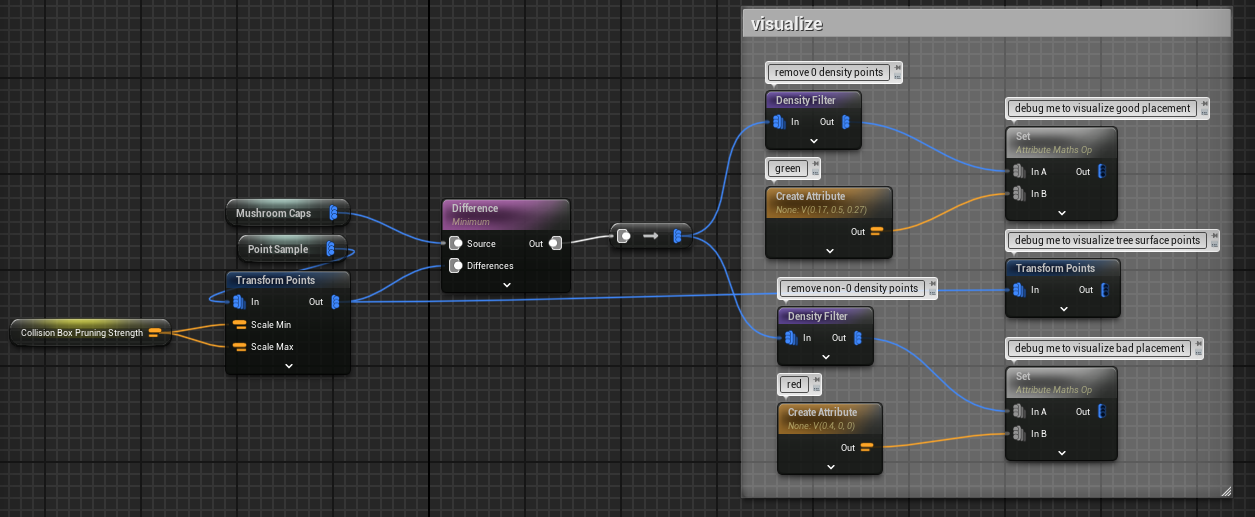
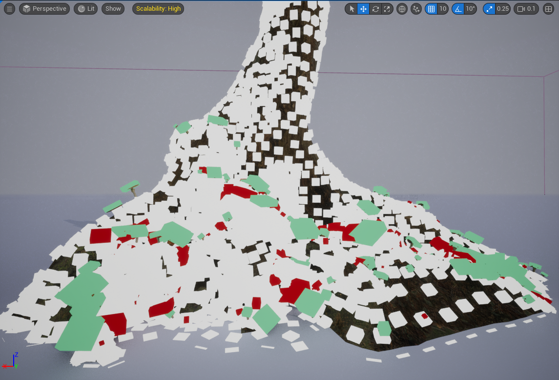
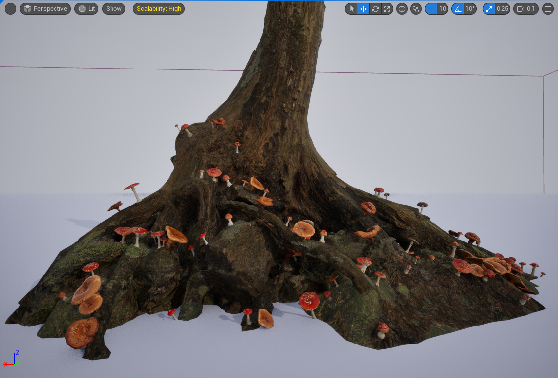
The Difference node is an important PCG node that allows you to remove certain points from a set of points based on the content of one or more sets of “difference” point data. A practical example of this in action is my mushroom generator project (see it here in my portfolio). In my PCG graph, I have a set of points that represent the caps of each mushroom, and I use the difference node cull mushrooms with caps that intersect with points sampled on the tree stump. In the image below, you can see the sampled tree points (in white), the mushroom caps that intersect with the tree stumps (in red), and the mushroom caps that are “good” i.e. no intersection (in green). So to put it another way: I use the difference node here to “subtract” the white cubes from the colored cubes. The red cubes are the ones that ended up getting subtracted, and the green ones are the ones that are left.
The final result:
Under the Hood
An important thing to understand about how the difference node works is that it doesn’t actually subtract points with identical positions from your source points. Instead, it samples points from each of the streams in the “differences” input, creates a union of those sampled points, and finally performs a subtraction between the source attributes and the union attributes. Let’s break each of these down individually:
How Point Sampling Works in PCG
When PCG performs a sample on point data, it uses a transform and a bounding box to get a collection of points that are clustered together within the bounding region. Then, it performs a weighted blend of the attributes on those points (position, rotation, scale, density, bounds, color, steepness). The weight is calculated based on how much the bounding box of the target point overlaps with the source point.
Union Data
The Union operation could probably warrant its own blog post, but in the interest of time, I will just give a brief explanation of how it functions. From my limited research, performing a union on multiple data streams will:
1) Pick the transform and bounding box of the first point it finds for each exact point position (no weighted blending). 2) Use that transform and bounding box to blend the attributes all other near points using the following rules: 1) Density is blended using the union density function (more on density functions below) 2) All other attributes are blended using a MAX operation (pick the largest value).
Subtraction
As opposed to the transform and bounding box (which are weight-blended) and density (which is blended using the density function - more on this below), the rest of the point attributes involved in the difference operation simply have their values subtracted.
Note: The subtraction step can be toggled on and off with the Diff Metadata option (see below for more info).
Concrete Example
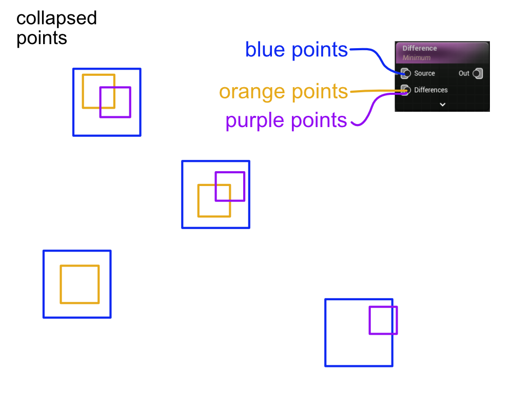
Consider the image below. In this example, I am “subtracting” the orange and purple points from the blue points. Under the hood, PCG will first individually sample from the orange point data stream and the purple data stream. In the case of the difference node, the sample uses the transforms and bounding boxes of the source points (blue) to decide which points should be grouped together in the sample.
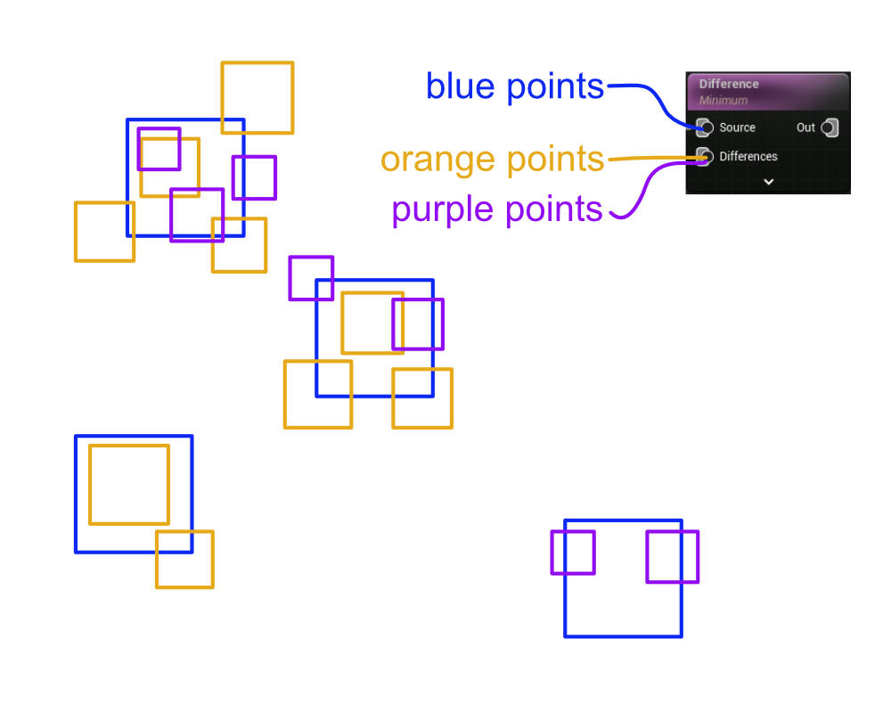
This means that for each blue point, a “collapsed” orange point and a “collapsed” purple point will be produced. These collapsed points will have attributes that are weighted by how much the un-collapsed points’ bounding boxes were overlapping with the nearest blue point bounding box.
NOTE: The image below is just an approximation of what I think the collapsed points would look like. I am fairly certain that in addition to the attributes being weight blended, the transforms and bounding boxes are weight blended as well. This would mean that when the individual differences streams are sampled, the collapsed points should basically have a transform position that is somewhere in the middle of the points that were combined, and this should have a bias towards points that are more “inside” of the source points’ (blue) bounding box. Just take this part with a grain of salt. I’m not 100% sure I have this correct.
Next, the two data streams are unioned together.
NOTE: Again, this is just my best guess as to what this would look like.
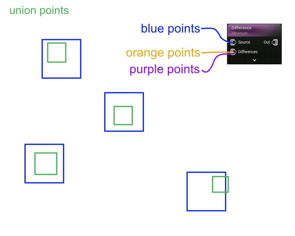
Lastly, the difference node actually subtracts the attribute values of the blue points with the union points. Note that attribute subtraction only actually happens if the density function is set to Minimum or Clamped Subtraction. More on this below.
Node Settings: Deep Dive
Density Function
Density is a bit of a special attribute for PCG point data. Fundamentally, it is just a float value, but it’s a special float value because it is often used to determine if a particular point should be culled or not. The difference node gives you several different options for how it computes the final density value of each point.
Minimum (Density Function)
The Minimum density function can be described as follows:
- density = source - Union(Diff0…Diffn, MAX)
Where MAX will take the maximum sampled density from streams Diff0…Diffn. So essentially this just says “subtract the near-point with the largest density”.
When to use
Use this one when you don’t care about how many points there are near the one you are subtracting from.
Clamped Subtraction (Density Function)
The clamped subtraction density function can be described as follows:
- = source - Union(Diff0…Diffn, CLAMPED_ADDITION)
Where CLAMPED_ADDITION will sum together all the sampled density values from each stream, with a max value of 1. So basically this causes each source point to have its density subtracted by the combined density of all the overlapping difference points.
When to use
Use this when you want the difference points to have a cumulative effect:
- i.e. source - difference = 0 more often when the difference stream has lots of near-points or those near-points have high density.
Binary (Density Function)
The binary density function can be described as follows:
- density = source - Union(Diff0…Diffn, BINARY)
Where BINARY will yield a density value of 1.0 if the sampled density value in any of the streams Diff0…Diffn is greater than 0. This results in a density value of 0.0 for each point being subtracted that has any density greater than 0.
When to use
This is probably the most commonly used density function. Use it when you basically want any overlapping points removed.
Mode
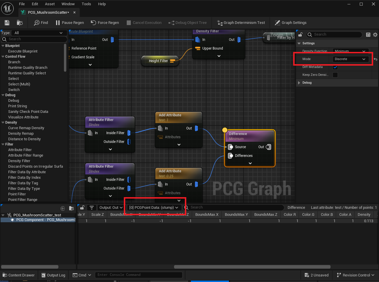
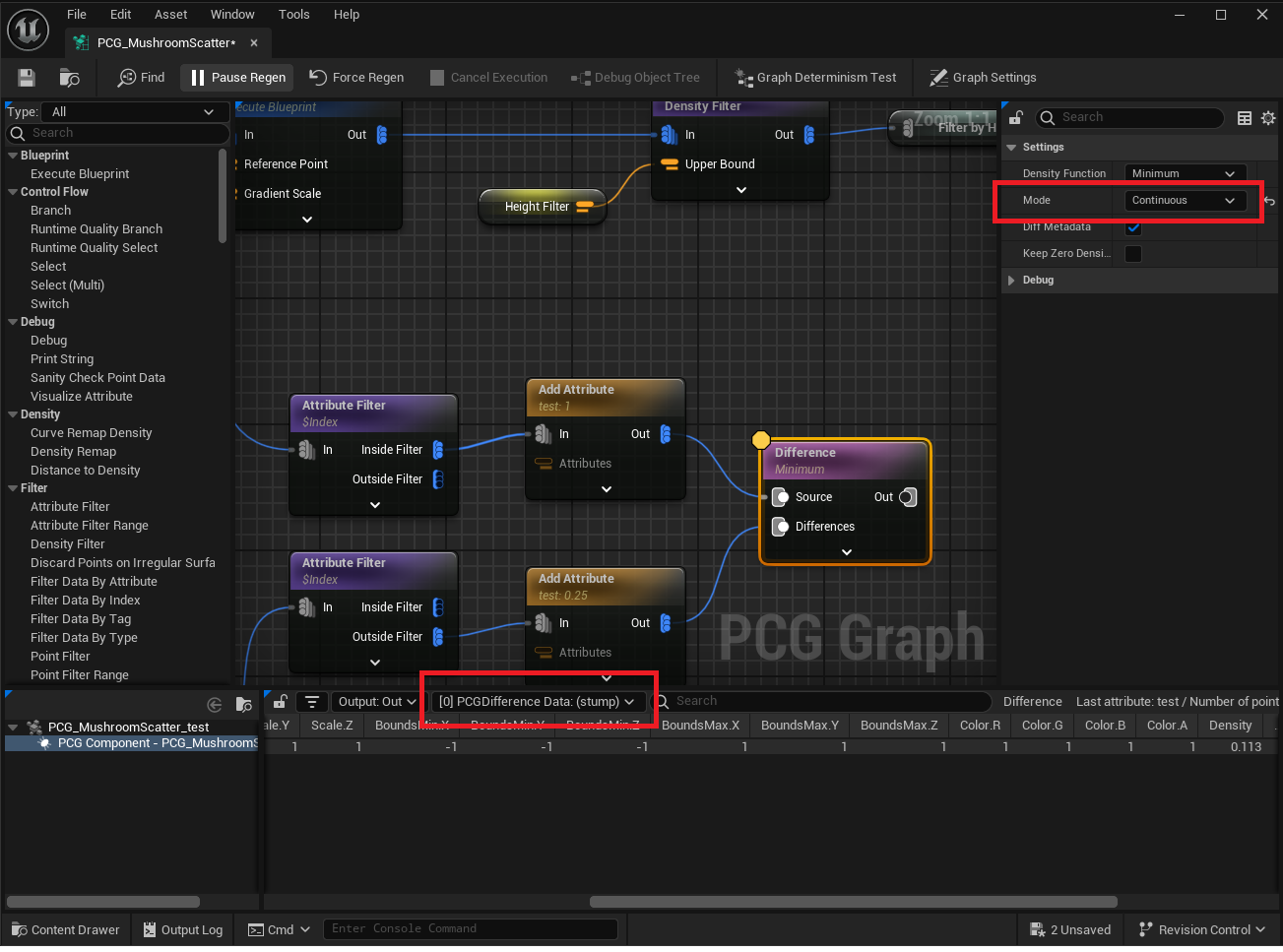
Mode just determines the output type of the difference node. You can see this in action by switching between Discrete and Continuous mode and looking at the node output in the inspection window:
Inferred Mode
Inferred mode uses Discrete mode if both the source input stream and at least one of the difference input streams are point data (i.e. of type UPCGPointData).
When to use
Probably almost always? Unless you have a good reason to explicitly set the mode, let the Unreal devs decide for you.
Continuous Mode
Continuous mode sets the output data type to just spit out the difference data directly. As far as I can tell, this means that every time the output of this node is sampled, it will re-run the difference computations, as opposed to Discrete mode, where those computations are computed once and then cached. Because of this, I believe continuous mode has SLOWER performance than Discrete mode. Not sure how much of a difference this makes though.
When to use
The only time you would use this is if you are computing this node on non-point data such as volume data, and you also want the output to be non-point data.
Discrete Mode
Discreate mode sets the node to output point data with all the difference computations cached.
When to use
I think the only reason you would explicitly use this mode is if you have a non-point data input and you want to force the output to be point data.
Diff Metadata
Diff Metadata simply controls if the attribute subtraction takes place or not.
NOTE: Diff Metadata doesn’t work when the density function is set to binary AND keep zero density points is set to true. This is because currently (as of UE5.5) the difference node code skips the subtraction computation when in binary mode. If keep zero density points is set to false, this doesn’t really matter, because you would expect that only points remaining will be ones that aren’t in proximity with other points- i.e. there is nothing to subtract from their metadata. However, when keep zero density points is turned ON, it still skips the metadata subtraction. It is unclear if this is a bug or working as intended.
When to use
Enable if you want the difference node to subtract attribute values.
Keep Zero Density Points
This setting is pretty straightforward. By default, this is DISABLED, meaning that any points with a density value of 0 will be removed from the output data. If you enable it, these points will be retained.
When to use
One useful reason for why you might want to enable this is for visualizing which points have been marked for removal by the difference node. I’ve learned the hard way that due to how the difference node samples points, if you do the following:
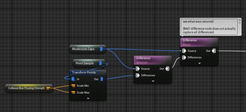
You are not actually guaranteed to get the points that were subtracted in that second difference node. Instead, it is much safer to just keep the zero density points and then filter them yourself using a density filter.
